Table of Contents
Previous: Lab 9
Intro
The goal of Lab 10 was to simulate localization of our cars in the pre-defined world using the Bayes filter.
Localization
Our cars don’t rely on localization, using sensor data and control inputs to estimate their position probabilistically, to navigate the world. This is done using a Bayes filter, which updates the robot's belief about its position as new data comes in.
The robot's state includes its position on the ground $(x, y)$ and its orientation ($\theta$). The ground plane is discretized into a grid with each cell representing a 1x1 ft space and 20° of orientation, resulting in a 12x9x18 state space.
Bayes Filter
The Bayes filter operates in two steps:
Prediction: The robot estimates its new position based on its previous pose and control inputs.
Update: The robot refines its estimate using sensor readings.
The motion model calculates the likelihood of the robot transitioning from one pose to another, while the sensor model calculates the probability of sensor observations given the robot’s position. The filter iterates over all possible poses in the state space to update the belief, and repeats for each move.
Lab Tasks
Per the notebook instructions, I wrote the following functions to simulate localization with the Bayes filter.
Control
I first wrote the compute_control() function, which takes the current and previous pose and returns the control input required to move from the previous to current. This forms the mean of a Gaussian distribution used to estimate the probability that the robot moved from its previous pose to the current one.
def compute_control(cur_pose, prev_pose):
    """ Given the current and previous odometry poses, this function extracts
    the control information based on the odometry motion model.

    Args:
        cur_pose  ([Pose]): Current Pose
        prev_pose ([Pose]): Previous Pose

    Returns:
        [delta_rot_1]: Rotation 1  (degrees)
        [delta_trans]: Translation (meters)
        [delta_rot_2]: Rotation 2  (degrees)
    """
    cur_x, cur_y, cur_theta = cur_pose
    prev_x, prev_y, prev_theta = prev_pose

    # Calculate the first rotation angle (in deg) before moving
    delta_rot_1 = np.arctan2(cur_y - prev_y, cur_x - prev_x) - prev_theta
    delta_rot_1 = np.degrees((delta_rot_1 + np.pi) % (2 * np.pi) - np.pi)  # Normalize the angle to [-pi, pi], convert

    # Calculate the translation
    delta_trans = np.sqrt((cur_x - prev_x)**2 + (cur_y - prev_y)**2)

    # Calculate the second rotation angle (in deg) after moving
    delta_rot_2 = cur_theta - prev_theta - delta_rot_1
    delta_rot_2 = np.degrees((delta_rot_2 + np.pi) % (2 * np.pi) - np.pi)  # Normalize the angle to [-pi, pi], convert

    return delta_rot_1, delta_trans, delta_rot_2
Motion Model
The odometry motion model gives information necessary for the prediction step of the Bayes filter: A state transition probability from the previous recorded pose to the current one. It does this knowing the current pose, previous pose, and actual vs. predicted control inputs (via compute_control()). The resulting transition probability is the product of the probabilities of each movement because they are executed in series.
    """ Odometry Motion Model

    Args:
        cur_pose  ([Pose]): Current Pose
        prev_pose ([Pose]): Previous Pose
        (rot1, trans, rot2) (float, float, float): A tuple with control data in the format
                                                   format (rot1, trans, rot2) with units (degrees, meters, degrees)


    Returns:
        prob [float]: Probability p(x'|x, u)
    """

    # Get control parameters from the current and previous poses
    d_rot_1, d_trans, d_rot_2 = compute_control(cur_pose, prev_pose)

    # Determine the probabilities of the control parameters
    pr_rot_1 = loc.gaussian(d_rot_1, u[0], loc.odom_rot_sigma)
    pr_trans = loc.gaussian(d_trans, u[1], loc.odom_trans_sigma)
    pr_rot_2 = loc.gaussian(d_rot_2, u[2], loc.odom_rot_sigma)

    return pr_rot_1 * pr_trans * pr_rot_2
Prediction
prediction_step() takes in odometry data and outputs the predicted belief $\overline{bel}$ of the robot's pose using the odometry model. It does this by iterating over each pose in the state space and calculating a transition probability for it using odom_motion_model().
We don't deal with states with a transition probability of less than 0.0001 to speed up computation. Because the probability distribution will converge to a small enough range to be useful in reasonably short time, we are probably safe in doing this. As a result, we lose a bit of compleness in Bayes filter execution, but gain a lot of time.
def prediction_step(cur_odom, prev_odom)
  # Initialize the predicted belief
  loc.bel_bar = np.zeros((mapper.MAX_CELLS_X, mapper.MAX_CELLS_Y, mapper.MAX_CELLS_A))

  # Iterate over state space
  for x_prev in range(mapper.MAX_CELLS_X):
      for y_prev in range(mapper.MAX_CELLS_Y):
          for theta_prev in range(mapper.MAX_CELLS_A):
              # Skip unlikely states
              if loc.bel[x_prev, y_prev, theta_prev] < 0.0001: continue

              # Loop through all possible current states
              for x_curr in range(mapper.MAX_CELLS_X):
                  for y_curr in range(mapper.MAX_CELLS_Y):
                      for theta_curr in range(mapper.MAX_CELLS_A):
                          # Calculate transition probability
                          p = odom_motion_model(
                              mapper.from_map(x_curr, y_curr, theta_curr),
                              mapper.from_map(x_prev, y_prev, theta_prev),
                              u
                          )

                          # Update predicted belief
                          loc.bel_bar[x_curr, y_curr, theta_curr] += p * loc.bel[x_prev, y_prev, theta_prev]

  # Normalize the belief
  loc.bel_bar = np.sum(loc.bel_bar)
Sensor Model
sensor_model() performs a similar function to our odometry motion model. Given a set of sensor observations at a pose, it returns the probability of that sensor observation.
def sensor_model(obs):
    """ Compute p(z|x), the likelihood of sensor measurements for a given pose.

    Args:
        obs (ndarray): 1D array of true sensor readings for a specific robot pose.

    Returns:
        ndarray: 1D array of size 18 (loc.OBS_PER_CELL) with sensor measurement likelihoods.
    """
    # Initialize the probability array
    prob_array = np.zeros(mapper.OBS_PER_CELL)

    for i in range(mapper.OBS_PER_CELL):
        # Calculate the likelihood of each sensor reading
        prob_array[i] = loc.gaussian(obs[i], loc.obs_range_data[i], loc.sensor_sigma)

    return prob_array
Update
As the final step in Bayes filter implementation, update_step() again iterates through all poses in the state space and updates the belief given the output of the sensor model (with sensor_model()) and predicted belief (updated in prediction_step()). It multiplies elements of the sensor model output for the final $$ p(z_t | x_t, m) = \prod_{k=1}^{18} p(z_t^k | x_t, m) $$
expression, and uses $p$ to to update the belief at each point before renormalizing the distribution.
def update_step():
    """ Update the belief (loc.bel) based on the predicted belief (loc.bel_bar) and the sensor model.
    """
    # Iterate over the grid to update the belief
    for x in range(mapper.MAX_CELLS_X):
        for y in range(mapper.MAX_CELLS_Y):
            for theta in range(mapper.MAX_CELLS_A):
                # Compute the sensor model likelihood for the current pose
                p = sensor_model(mapper.get_views(x, y, theta))

                # Update the belief for the current state
                loc.bel[x, y, theta] = np.prod(p) * loc.bel_bar[x, y, theta]

    # Normalize the belief distribution
    loc.bel /= np.sum(loc.bel)
Execution
Video
I recorded the first execution of the filter. Further executions are below.
Screenshots
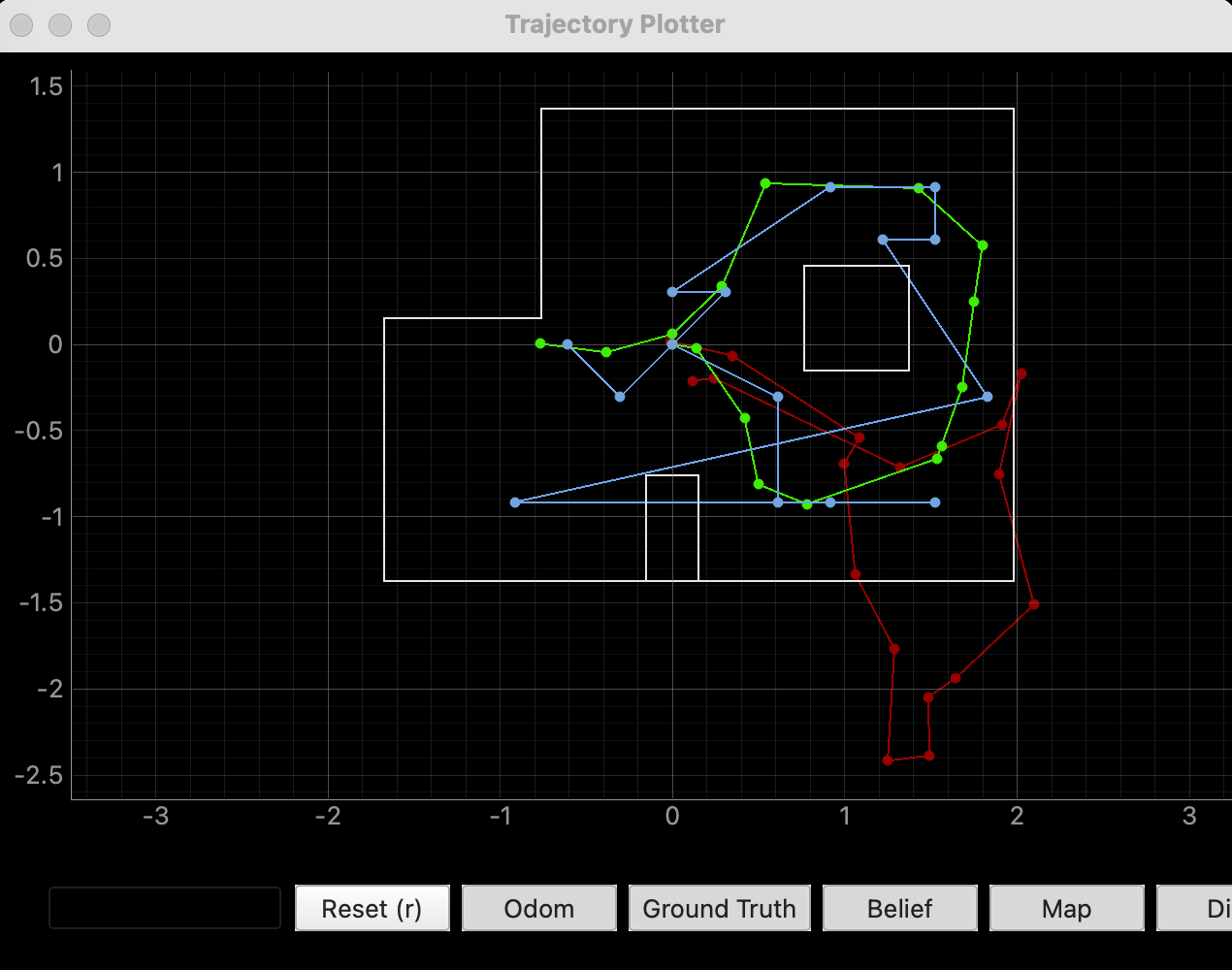
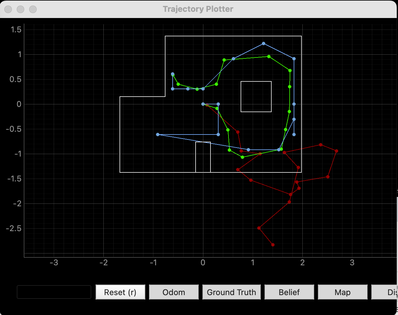
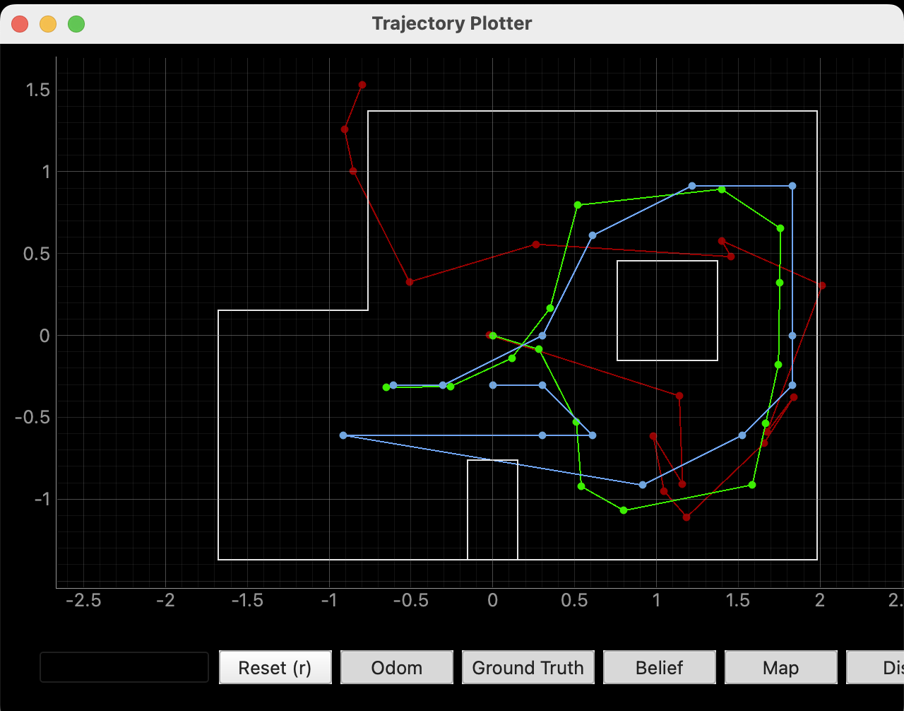
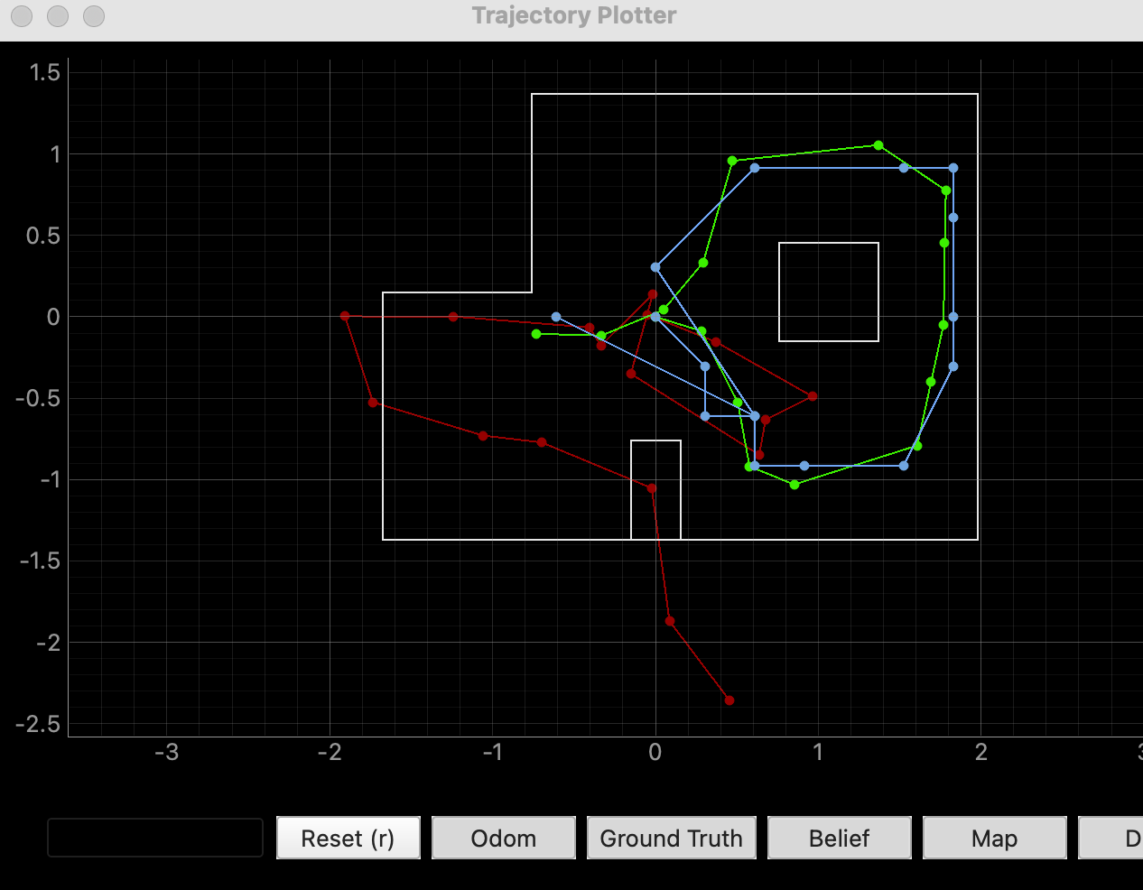
There was more variability in the estimates than I expected, especially in open spaces where sensor data (even simulated) is less reliable. Still, they're miles better than the pure odometry model.
Collaborations
I worked with Lucca Correia and Trevor Dales extensively. I referenced Stephan Wagner's and Mavis Fu's sites for code examples.