Previous: Lab 10

Intro

The goal of Lab 11 was to demonstrate real-world localization of the robot based on our simulations from Lab 10. We were provided optimized localization code and asked to build a way for our robots to collect the required data.

Lab Tasks

Simulation

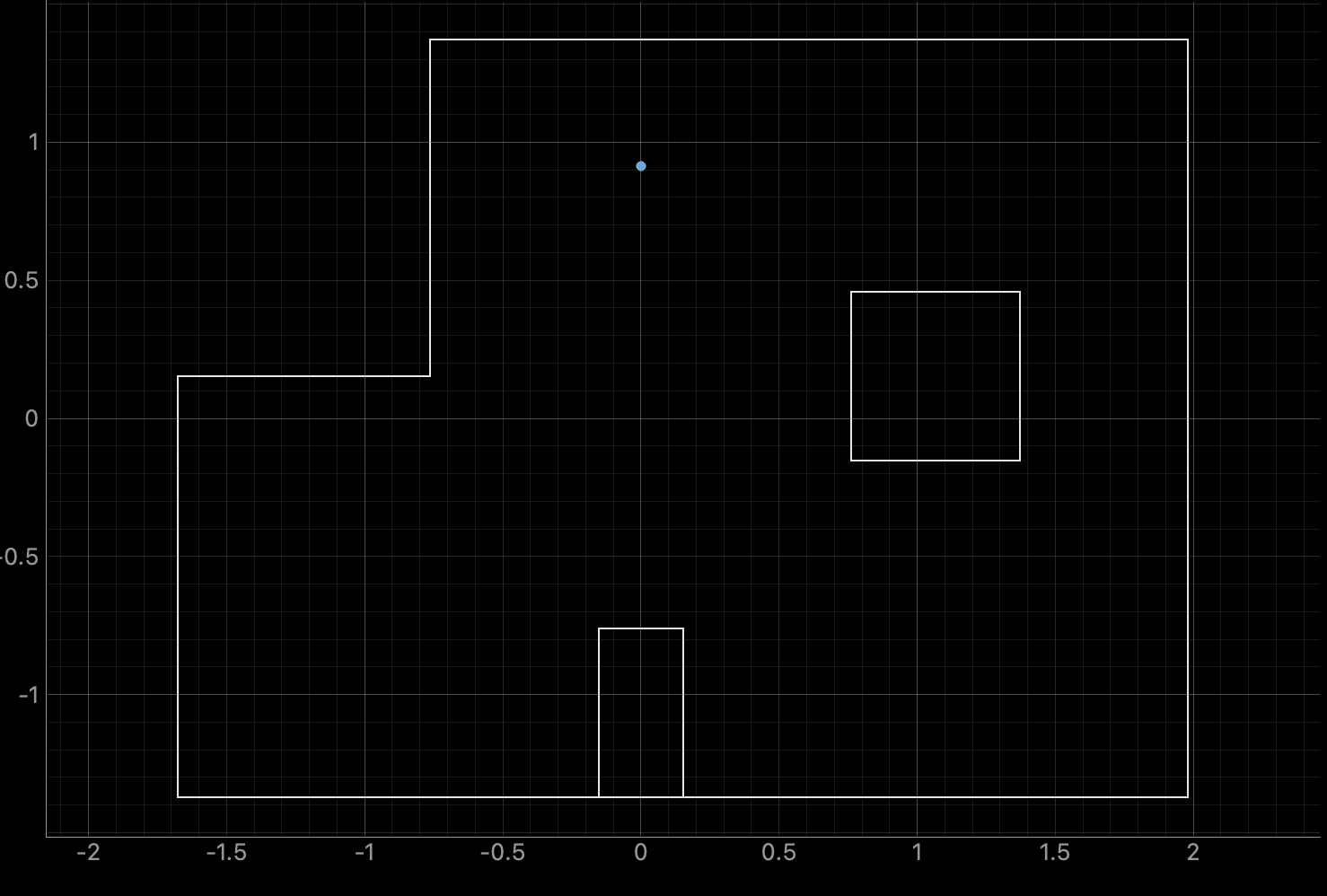
I ran the simulated localization from Lab 10 again and got the following response.

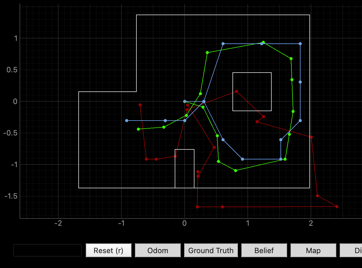
    Clearly, odometry is unreliable and we must make a more informed estimate about our robot's state. To do this, we can perform a 360 degree spin about the robot's axis and get TOF data, just like we simulated in lab 10. In this case, we're just performing the update step as prediction doesn't get us much with inaccurate models of our robots.

Updating

I primarily used my mapping code from Lab 10 to implement the update step, reusing arrays from lab 7 to save memory. It takes 18 sets of distance measurements at 20 degree angles and sends the data back over BLE. These measurements are parsed from the notification handler into a CSV and processed by the provided localization code.

case START_MAP:

    doMap = 1;
    success = robot_cmd.get_next_value(map_interval);
    if (!success) return;
    // start TOF ranging
    distanceSensor1.startRanging();
    distanceSensor2.startRanging();

    target_orientation = 0;
    digitalWrite(blinkPin, HIGH); // visual indicator
    for(int i = 0; i<=18; i++){

        start_time_map = millis();
        while(millis() - start_time_map < map_interval){  // approx settling time of 20 deg move

        // record TOF
        if (distanceSensor2.checkForDataReady()){
            distance2 = distanceSensor2.getDistance();
            pid_tof[pid_c] = distance2;
        }

        record_IMU(); // store DMP yaw to global var
        pid_orientation_tof(); // do orientation PID with recorded yaw
        apply_pid(); // drives motors according to type of control (pos, ori, or both)

        pid_c++;

        delay(10);
        
        }
        target_orientation = target_orientation - 20; // set up next measurement (counterclockwise)
    }
    digitalWrite(blinkPin, LOW); // visual indicator
    
break;

    But this system measures many distances at each reference angle, so I wrote a python script that picks the distance value at each measured angle that's closest to the reference. it's called at the end of perform_observation_loop to filter the incoming data. This filter gives the best distance at each reference angle, rather than a random one (i.e. polling the TOF only once at each angle). It takes in the filepath (str) of the CSV file output by the notification handler, and returns two column numpy arrays of TOF distances and reference angles at wich these readings were taken.

def compute_sensor_readings(filepath):

    # Read CSV
    df = pd.read_csv(filepath)

    ref_angles = np.arange(20, 361, 20).reshape(-1, 1)

    closest_values = []
    for angle in angles_flat:
        # compute circular difference between each yaw and the reference 
        yaw = df['yaw_value']
        diff = np.abs((yaw - angle + 180) % 360 - 180)
        # index of row with smallest difference
        idx = diff.idxmin()
        closest_values.append(df.at[idx, 'distance_value'])

    # shape into col vectors
    sensor_ranges   = np.array(closest_values).reshape(-1, 1)
    sensor_bearings = angles_flat.reshape(-1, 1)

    return sensor_ranges, sensor_bearings

This allows us to construct perform_observation_loop(), which signals the robot via BLE and feeds collected data into the previous filter. It is called within the Localization.get_observation_data() method, and outputs the same as the above filter.

    async def perform_observation_loop(self, rot_vel=120):

        with open('loc_data.csv', 'w') as f:
            f.truncate()

    
        ble.start_notify(ble.uuid['RX_STRING'], pid_handler)
        print("Started notifications.")


        #ble.send_command(CMD.ZERO_DMP, "")
        ble.send_command(CMD.SET_PID_GAINS, "2|.5|0.00001|0") # structure: 2 = orientation PID, Kp, ki, kd
        
        
        #ble.send_command(CMD.ZERO_DMP, "") # start at 0 angle
        
        ## initial setup, let orientation cook for a sec
        ble.send_command(CMD.SET_PID_TYPE, "2") # 1 = position, 2 = orientation, 3 = both
        ble.send_command(CMD.START_PID, "100|0|1") # position setpoint, orientation setpoint, record y/n
        await asyncio.sleep(1)
        ble.send_command(CMD.STOP_PID, "") 
        
        ## initial setup, let orientation cook for a sec
        ble.send_command(CMD.SET_PID_TYPE, "2") # 1 = position, 2 = orientation, 3 = both
        ble.send_command(CMD.START_MAP, "500") # start map with mapping interval of 500 ms

        print("starting map")

        await asyncio.sleep(20) # wait for map complete 


        # record data
        ble.send_command(CMD.SEND_PID_DATA, "") 

        print("sending data")

        await asyncio.sleep(30) # wait for csv complete


        file_path = "loc_data.csv"

        ranges, bearings = compute_sensor_readings(file_path)

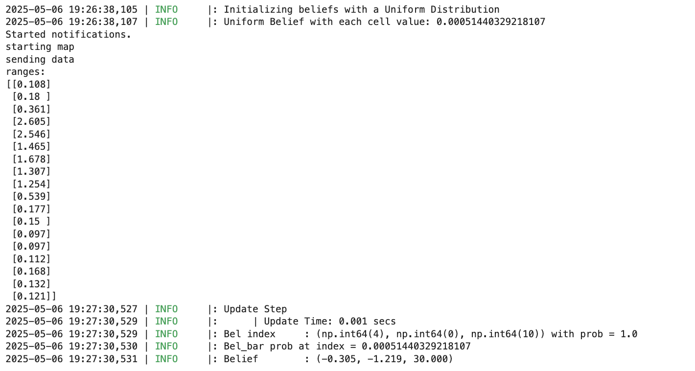
        print("ranges:")
        print(ranges)

        return ranges, bearings

Measurements

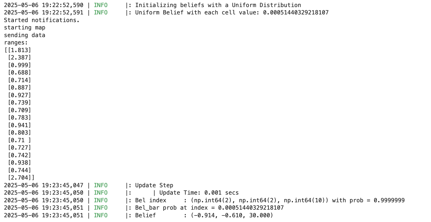
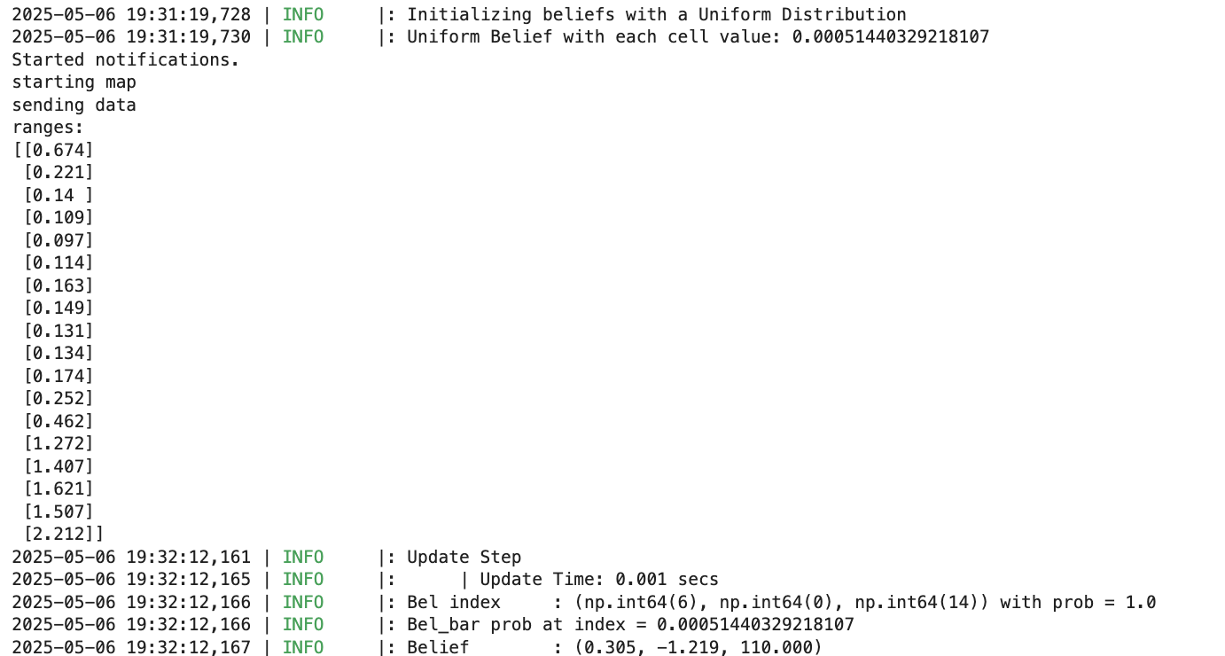
    This implementation got me the following set of distances at (5,-3) (I began oriented towards the lab) after a few test-runs of localization:

(5, -3)

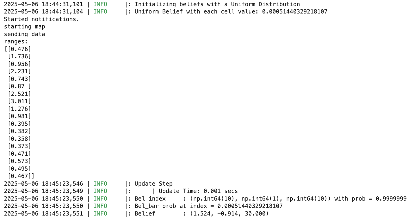
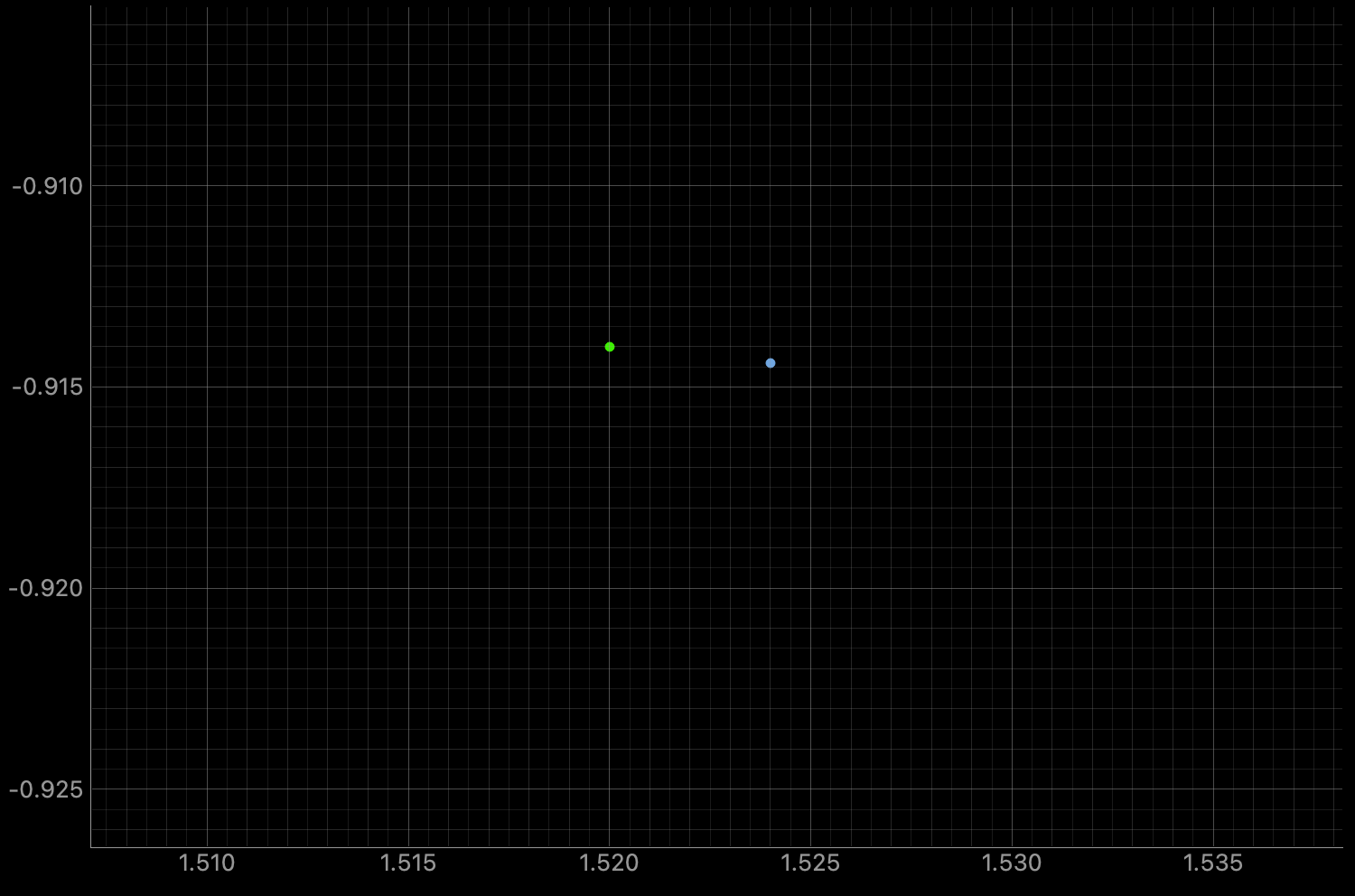
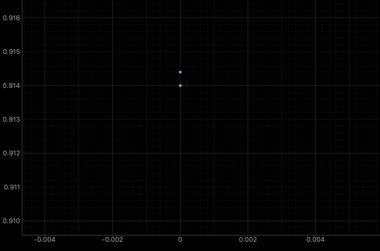
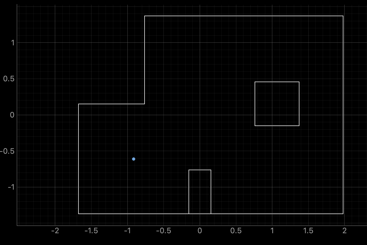
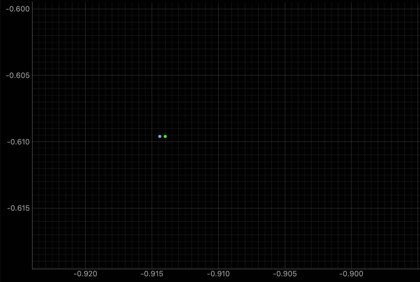
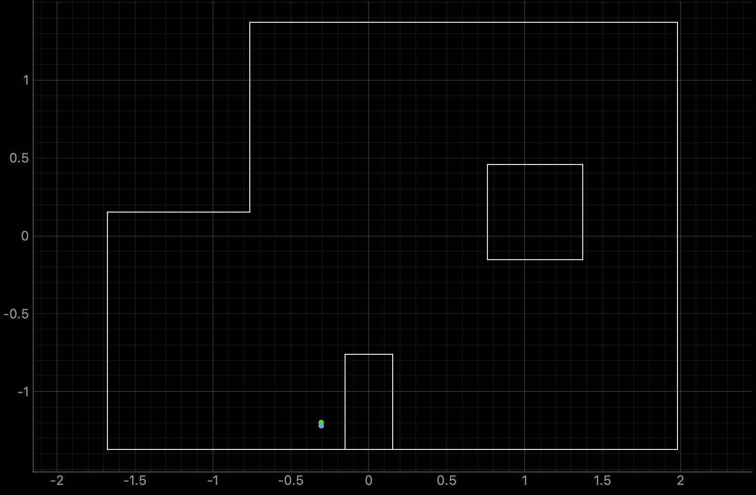
    The final localization output is plotted below (blue) with ground truth (green). The distance between these points seems a bit too good to be true. I'm really not sure how it localized so well with the datapints given.

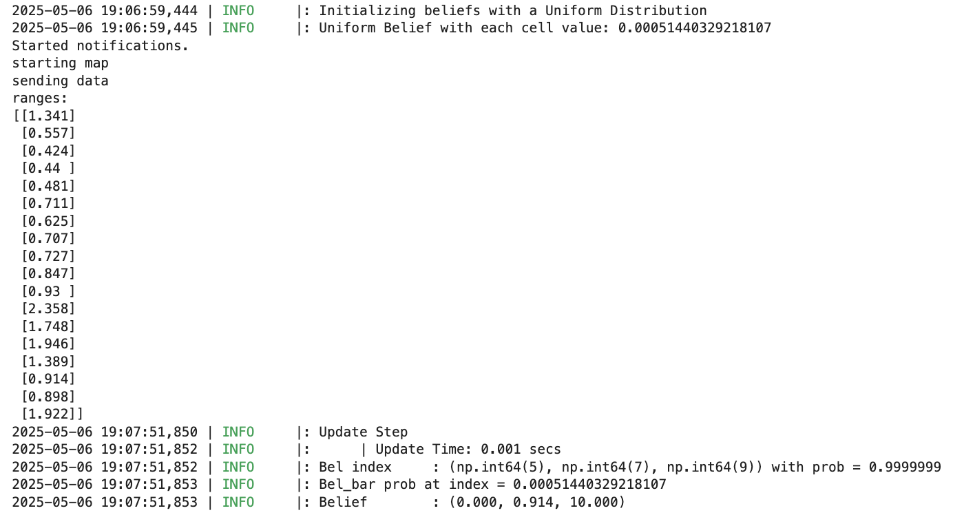
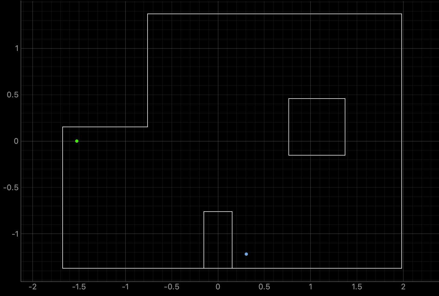
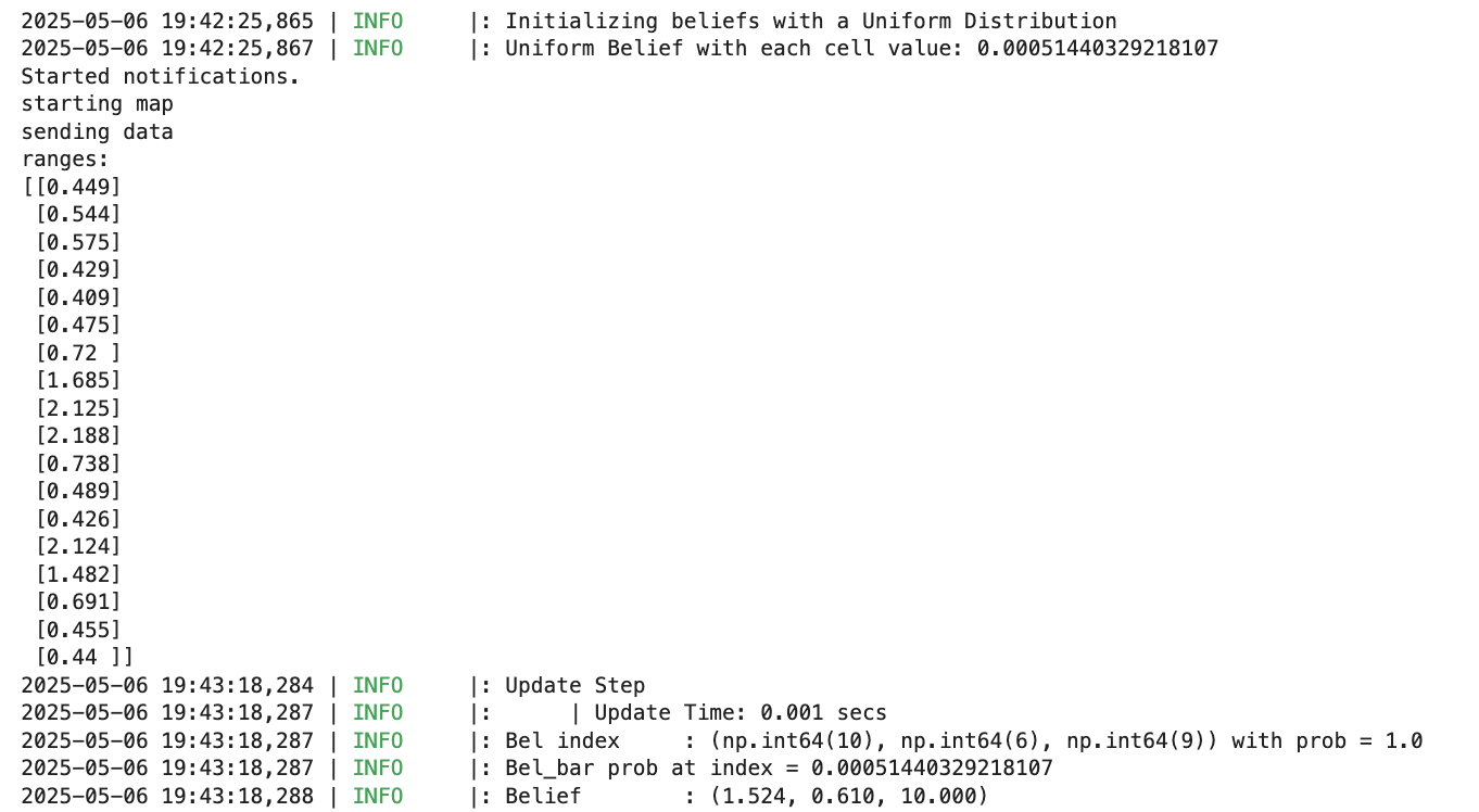
I localized at the remaining points and was also a bit shocked with the accuracy of the x and y estimate, given that angle estimates were fairly varied. The localization was almost 100% correct to ground truth for multiple consecutive runs at different points, except for at (5, 3):

(0, 3)

(-3, -2)

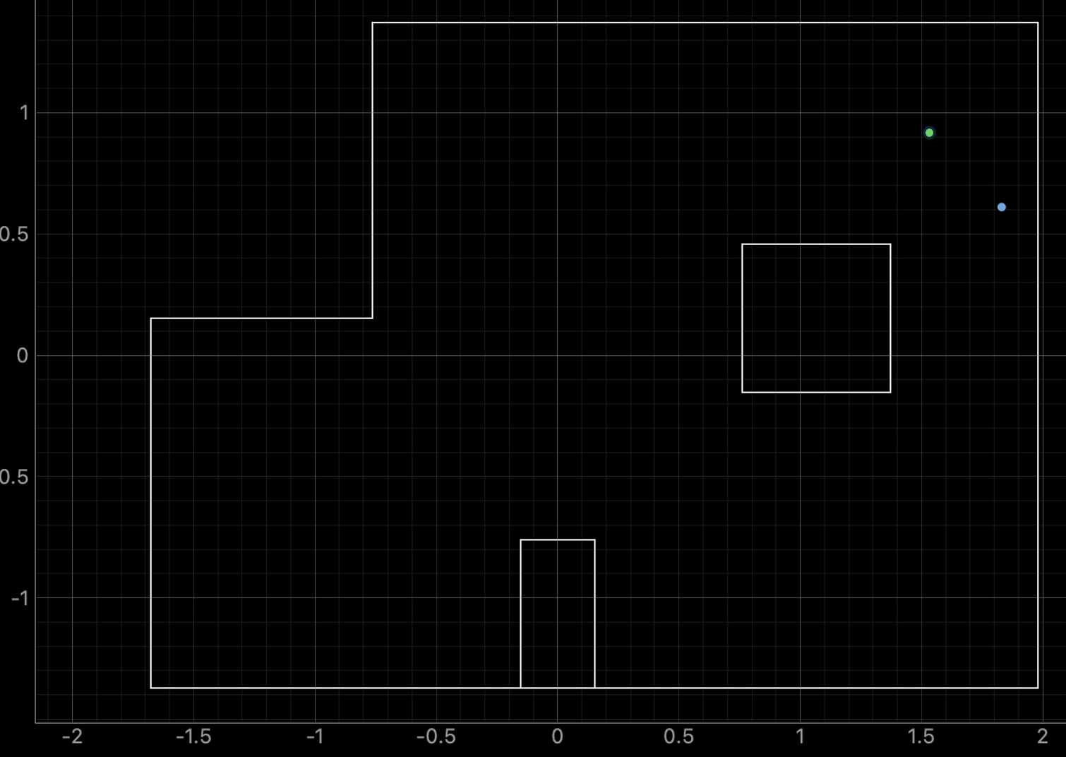
(5, 3)

At (5, 3), the filter seemed more uncertain. Estimates flip-flopped between the following two points. My thought was that the robot struggles most when close to interior corners connecting long walls, as much of the map is made up of them (note: I plotted the ground truth point in Powerpoint after the fact because I forgot to do so in lab).

I attempted to validate this hypothesis by placing the bot at (-5, 0) and localizing.

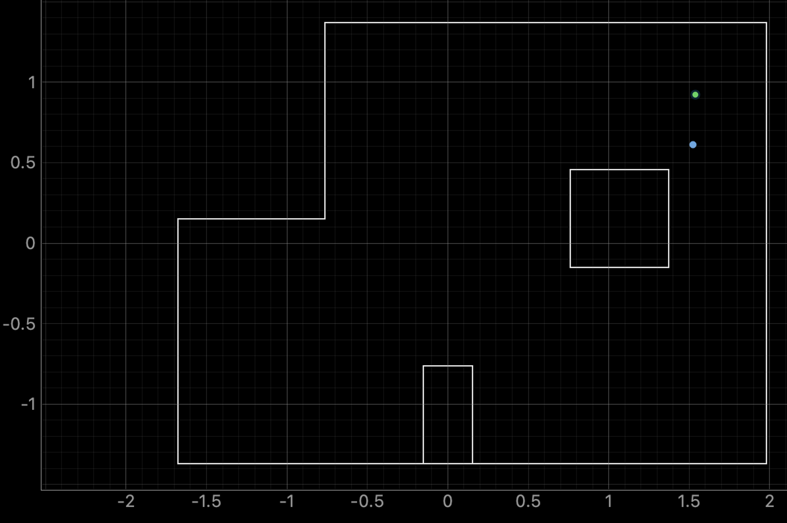
No problems here. I tried again with (0, -5) ft, which I knew looked similar to (1, -4) ft at a +90 degrees from the previous lab.

Bingo. The Bayes filter finally decided on the wrong point. I think this might have caused the issue with (5, 3). It must look similar to a couple of points in the same direction (in the pose space) from (1.524, 0.910, 0) (m, m, rad) as the two predicted points.

After all that, though, I ended up getting a good read from the top right:

Discussion

I'm really not sure what higher power blessed me with these values, but I'd be happy to run it again if any TA would like to verify. Either I got really lucky, or my filtering technique worked surprisingly well.

I did come upon an interesting limitation of the Bayes filter with real-world buildings and low-quality TOFs, though. Corners with similar(ly long) walls on either side end up looking similar enough to the filter to be mistaken.

Collaborations

I worked with Lucca Correia and Trevor Dales extensively. I used ChatGPT to help me with my distance data filter.

Next: Lab 12