Table of Contents
Previous: Lab 11
Intro
I worked with Lucca and Trevor Dales to navigate our robot through a preset route of waypoints assigned to us in the lab. Overall, we were very successful in arriving and navigating through these waypoints completely autonomously with a combination of onboard PID control and offboard localization with the Bayes filter! The final result was incredibly rewarding as it required us to combine and implement various aspects of code and hardware debugging learned throughout the semester in addition to navigation and waypoint logic for this lab. Note that we also considered an obstacle avoidance algorithm, but ran out of time to implement it within our lower-level control loop. This might have made our robot less robust to outside disturbances, but our navigation was still accurate within the lab.
We began with complementary arrays of waypoints and localization booleans (i.e. a point, and a boolean to signal the script to localize at that waypoint). This allowed us to manually assign which points we localized at based on the accuracy of localization at each waypoint for the most accurate navigation. To navigate between points, we used sequential orientation and position PID using the DMP onboard our IMU, and Kalman-filtered TOF sensor, respectively.
We used Lucca’s robot for this lab, and collaborated jointly on both Arduino and Python code components!
Goal Waypoints
Logic and Control Flow
The navigation path is defined by a list of 2D waypoints waypoint_list, with each point representing a target location in feet. An accompanying list of boolean flags localize_flags determines whether the robot should re-localize its position at each waypoint using a grid-based localization system. The script continuously loops through all waypoints in sequence, executing the following steps for each:
1. Turn Toward the Next Waypoint
Calculates the angle between the robot’s current position and the next waypoint using the
atan2function.Sends an angular PID control command over BLE to rotate the robot to the calculated heading (
CMD.PID_TURN_CONTROL, described in Onboard Control section)
2. Read Current TOF Sensor Data:
Requests the current pose from the robot (
CMD.SEND_CURRENT_POSE, which serves position data from the TOF over BLE).Extracts the distance reading from the CSV.
3. Move Toward the Waypoint:
Computes the expected distance to the next waypoint based on current position belief, and knowing that the robot's angle is always zero after mapping.
Subtracts the distance to the next point from the current TOF reading to calculate the necessary target distance for the next motion.
Sends a PID control command over Bluetooth to move the robot forward to the calculated target. (
CMD.PID_CONTROL, described in Onboard Control section)
4. Update Robot Location:
- If localization is enabled for the current waypoint, the robot turns to zero degrees and then performs an observation scan (function
perform_observation_loop) and sends the data through BLE. Then, an update step is performed to estimate the robot’s current position. - If localization is disabled, the robot’s position is assumed to be exactly at the waypoint.
- Note that the angle of the robot is always measured with the DMP from the horizontal (start) position as we found this to be significantly more accurate than any estimate from the Bayes filter, even with inconsistencies in how we started each test run.
Python Implementation
To realize the above plan, we wrote the following script.
async def recieveData(localizing, current_waypoint):
# return current location, current orientation
current_loc = [0, 0]
print("localizing: ",localizing)
if localizing:
await loc.get_observation_data()
# Run Update Step
loc.update_step()
belief = loc.plot_update_step_data(plot_data=True)
current_loc[0] = 3.281*belief[0] # x
current_loc[1] = 3.281*belief[1] # y
else:
#assume we are at the waypoint
current_loc = [current_waypoint[0], current_waypoint[1]] #set current location to x,y of the current waypoint
cmdr.plot_bel(current_waypoint[0]/3.281, current_waypoint[1]/3.281)
return current_loc
def calculateTargetAngle(x, y, next_waypoint):
# based on current location, calculate and return required angle
x2 = next_waypoint[0]
y2 = next_waypoint[1]
angle_rad = math.atan2(y2 - y, x2 - x)
target_angle_deg = math.degrees(angle_rad)
return target_angle_deg
def calculateTargetDistance(x, y, current_tof, next_waypoint):
#Implement logic
x2 = next_waypoint[0]
y2 = next_waypoint[1]
distance_to_next_waypoint = math.sqrt((x2 - x)**2 + (y2 - y)**2)
distance_to_next_waypoint = distance_to_next_waypoint*304.8 #convert from ft to mm
target_distance_mm = current_tof - distance_to_next_waypoint
return target_distance_mm
# Reset Plots
cmdr.reset_plotter()
# Init Uniform Belief
loc.init_grid_beliefs()
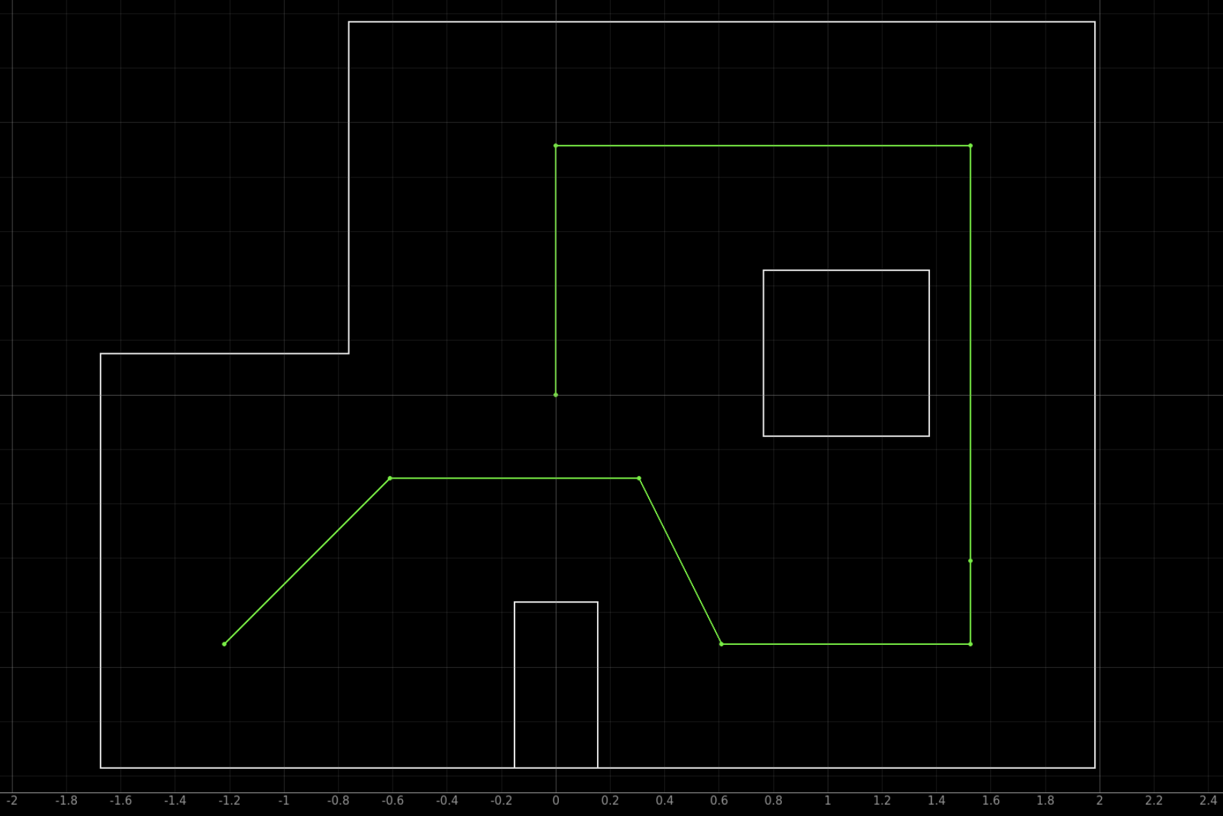
waypoint_list = [(-4, -3), (-2, -1), (1, -1), (2, -3), (5, -3), (5, -2), (5, 3), (0, 3),(0, 0)]
localize_flags = [False, True, False, False, False, True, True, True, True] # encode whether to localize at a waypoint
current_loc = [-4,-3] #initialize starting loc as the first waypoint
current_tof = 0 # [mm]
cmdr.plot_bel(current_loc[0]/3.281, current_loc[1]/3.281)
while True:
for i in range(len(waypoint_list)): # i represents current waypoint (starts at zero)
target_angle = calculateTargetAngle(current_loc[0], current_loc[1], waypoint_list[i+1])
print("Target angle:", target_angle)
ble.send_command(CMD.PID_TURN_CONTROL, f"1.1|0|120|{target_angle}") # P|I|D
await asyncio.sleep(5)
ble.send_command(CMD.SEND_CURRENT_POSE, "")
await asyncio.sleep(1.0)
df = pd.read_csv("MappingData.csv")
current_tof = df["TOF"].iloc[0]
print("Current TOF:", current_tof)
target_distance = calculateTargetDistance(current_loc[0], current_loc[1], current_tof, waypoint_list[i+1])
print("Target Distance:", target_distance)
ble.send_command(CMD.PID_CONTROL, f".14|0|40|{target_distance}") # P|I|D
await asyncio.sleep(10.0)
current_loc = await recieveData(localize_flags[i], waypoint_list[i+1])
print("Current Location:", current_loc)
with open("MappingData.csv", "w") as f:
f.truncate()
print("------------------------------------------------------------")
All BLE commands are explained below.
Onboard Control
Note that all data sent over from the Artemis to the computer over BLE is processed and piped into a CSV file by a notification handler. This CSV file is reset at specific points throughout the Python script before new TOF and Gyro data comes in.
Initially, an arrived boolean flag (triggered when the robot arrived within a threshold of the target angle or distance) was used to end the PID control and move to the next step in our larger control loop. However, this meant that if we slightly overshot the target, the flag would flip true and disable the control required to return to the target.
We tried to severly overdampen both orientation and linear PID to fix this, however it left us with too much steady-state error given the variability of our deadband with battery voltage.
Our solution was implementing a simple 5 second cutoff timer before stopping the PID loop. While not the most elegant solution, this gave us plenty of time to approach angles/distances and eliminated the issue of early PID stoppage. getDMP(), RunPIDLin(), and RunPIDRot() are well-documented in previous labs, and handle the lowest level of data acquisition, filtering, and motor control. The clearVariables() function is seen in all cases used in this lab; it resets counters and recorded datapoints to ensure the Artemis doesn't run out of memory over long execution times.
For angular PID, we used:
// Get PID parameters over BLE
success = robot_cmd.get_next_value(Kp_turn);
if (!success) return;
// Same for Kd & Ki
...

success = robot_cmd.get_next_value(target_turn);
if (!success) return;
tx_estring_value.clear();

// Variables used for cutoff timer (5 s)
...

int turn_cutoff = 5000;
while ( (millis() - turn_starttime) < turn_cutoff ) {
    getDMP();
    runPIDRot();
    counter_turn += 1;

}
stop();
pidTurn_start = 0;
clearVariables();
break;
and for linear PID:
distanceSensor1.startRanging();
pid_start = 0;
// Get PID parameters over BLE
success = robot_cmd.get_next_value(Kp);
if (!success) return;
// Same for Kd & Ki
...

success = robot_cmd.get_next_value(target_tof);
if (!success) return;
tx_estring_value.clear();

// Variables used for cutoff timer (7 s)
...
int linear_cutoff = 7000;

while ((millis() - linear_starttime) < linear_cutoff) { // hard time cutoff
    runPIDLin();
    counter_lin = counter_lin + 1;
}
    stop();
    clearVariables();
    run = 0;

    break;
We performed our mapping in a case outside of the mainloop for simplicity. It's taken mostly from lab 11, but implements the same changes as above (adding a timer) to improve robustness at the cost of speed.
case SPIN:{
    distanceSensor1.startRanging();
    success = robot_cmd.get_next_value(Kp_turn);
    if (!success) return;
    success = robot_cmd.get_next_value(Ki_turn);
    if (!success) return;
    success = robot_cmd.get_next_value(Kd_turn);
    if (!success) return;

    // Time varaibles
    spin_time = millis();
    start_time_pid_turn = millis();
    last_rotation_time = millis();

    while ((spin_counter < spin_len) && (rot_counter <= 36)) {

        getDMP();
        runPIDRot();

        spinTime[spin_counter] = millis() - spin_time;

        elapsed_time = millis() - last_rot_time;

        if ((start_time - millis()) < 750) {
            collectTOF();
            last_rot_time = millis();
            rot_counter = rot_counter + 1;
            target_turn = target_turn + 10;
        }
        spin_counter = spin_counter + 1;
    }
    stop();
    sendMapData();
    break;
}
Results
Below are a series of trials from our lab! In the last two runs you can see a live belief map and logging in Jupyter Notebook, which ouputs critical information like whether we localize at that specific waypoint, our current belief pose, our calculated target heading, etc. Note that we chose points to localize that the robot was least consistent in reaching, and left other points entirely up to the lower-level-control.
We saw a lot of success with the structure of our high-level planning on the first run, but ran into trouble with inconsistencies in lower-level control and angle targeting. When we localized, our planner output was correct based on position belief, but we struggled to tune the orientation PID loop in such a way that it responded (similarly) well to changes in angle between 10 and 180 degrees, while settling within a reasonable time. We changed our approach to add a time cutoff to both control loops, sacrificing a bit of accuracy for longer-term operation.
Note: We had to to nudge the robot at (-5,-3) to keep it on track as the TOFs appeared to slightly overestimate the target distance, which would have led to our robot crashing into the square obstacle. We also had some of the same issues with lower-level orientation control (unprecidented derivative gain) during mapping at (5,3), which we had to manually fix. Otherwise, this run was almost a complete success!
Here's the money shot. After all of our modifications, the robot was finally able to plan and execute a complete circuit around the world autonomously. Although each point wasn't reached with complete accuracy (see (5, 3)), the Bayes filter was able to bridge the gap and keep our robot on track throughout the run.
Collaborations
I worked with Lucca Correia and Trevor Dales to complete this lab with Lucca's robot. We used ChatGPT to verify Python implementation of our geometry for the high-level path planning. I also want to shoutout Kobe, who provided extreme moral support throughout this lab.