Previous: Lab 6

Lab Tasks

System Identification

If we approximate the open-loop robot system as first-order with respect to velocity, using Newton's second law to write

$$ F = ma = m\ddot{x} $$

with dynamics

$$ \ddot{x} = \frac{d}{m} \dot{x} + \frac{u}{m} $$

where $d$ and $m$ are lumped-parameter terms to roughly describe the drag (incorporating resistance from the air, ground, and motor dynamics) and intertia (incorporating mostly car mass, but also motor dynamics).

Choosing a state

$$ x = \begin{bmatrix} x \cr \dot{x} \end{bmatrix} $$

we can then describe the open-loop system in state-space form as $$ A = \begin{bmatrix}0 & 1 \cr 0 & -d/m\end{bmatrix} \text{ } B = \begin{bmatrix}0 \cr 1/m\end{bmatrix}. $$

We're only directly measuring the TOF data $x$, so it makes sense for our state-space system to output exclusively the position of the system (relative to a wall). In other words, with transition and output matrices

$$ C = \begin{bmatrix} -1 \cr 0 \end{bmatrix} \text{ } D = \begin{bmatrix}0 \cr 0\end{bmatrix} $$

With a PWM input of 80 (around the center of my applied range in Lab 5), I measured the following open-loop data and applied a low-pass-filter with $\alpha$ = 1 Hz:

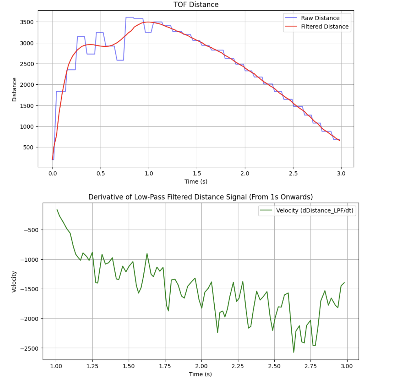
I then applied an exponential fit to the velocity data and marked the steady-state and 90% rise time points.

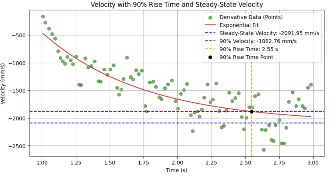
with a steady-state velocity of -2091.5 mm/s $\approx$ -2.09 m/s, and 90% rise time of 2.55 s, and setting u = 1 N (unit input), we have

$$ d = \frac{1 N}{2.09 m/s} = .478 kg/s $$

as our drag parameter, and

$$ m = \frac{.478 kg/s * 2.55 s}{ln(.1)} = .529 kg $$

as our momentum parameter, leading to

$$ A=\begin{bmatrix}0 & 1 \cr 0 & -0.903\end{bmatrix}
$$

and $$ B=\begin{bmatrix}0 \cr 1.75\end{bmatrix} $$

Note: looking back on this, I used too low a speed compared to my maximum for a 90% rise time -- I should've used something like 60%. However, my filter performed well with the above values, so I decided to proceed without going back and modifying A and B.

Kalman Filter Simulation

I get new motor inputs (not necessarily new TOF values ) every 20 ms, so I used that as my Kalman filter timestep.

to get an initial estimate for variances, I used

$$ \sigma_1 = \sigma_2 = \sqrt{\frac{100}{dt}} $$ for the process uncertainty, based on the sample time $dt$ that the system has to deviate from the predicted state, and $$ \sigma_3 = \sqrt{\frac{100}{dx}} $$ for the sensor uncertainty, based on the sensor variance $dx$. In a static test at 2000 mm from a white wall, I measured a variance $dx = 80.9$ mm.

Substituting,

$$ \sigma_1 = \sigma_2 = 70.7 $$ and $$ \sigma_3 = 35.1. $$

I then discretized my matrices according to the above $dt = .02$ s and used the provided kf() to filter my data in Python.

Ad = np.eye(2) + dt * A
Bd = dt * B

x = np.array([[-tof[0]], [0]])  # TOF from collected data

Sigma_u = np.array([[sigma_1**2, 0], [0, sigma_2**2]]) # process noise
Sigma_z = np.array([[sigma_3**2]]) # sensor noise

...


def kf(mu, sigma, u, y):
    mu_p = Ad.dot(mu) + Bd.dot(u)
    
    
    sigma_p = Ad.dot(sigma.dot(Ad.transpose())) + Sigma_u
    
    sigma_m = C.dot(sigma_p.dot(C.transpose())) + Sigma_z
    
    kkf_gain = sigma_p.dot(C.transpose().dot(np.linalg.inv(sigma_m)))
    
    y_m = y - C.dot(mu_p)
    
    mu = mu_p + kkf_gain.dot(y_m)
    
    sigma = (np.eye(2) - kkf_gain.dot(C)).dot(sigma_p)
    

    return mu, sigma

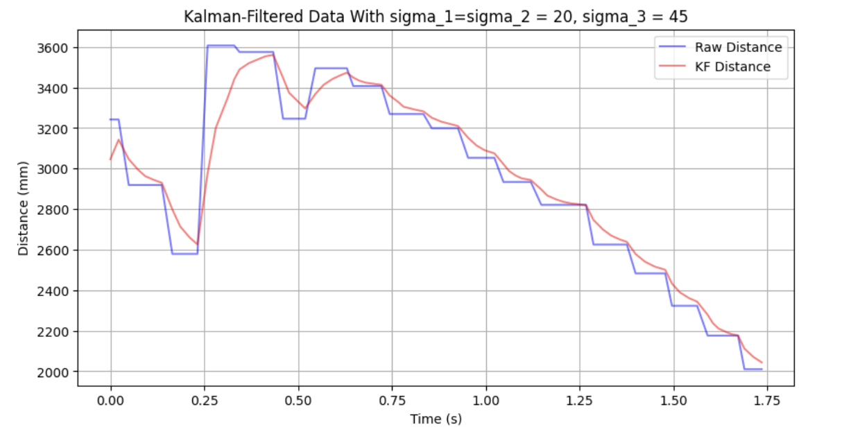
With my process and sensor noise of $\sigma_1 = \sigma_2$ = 70.7 and $\sigma_3$ = 35.1, my filtered data looked like this:

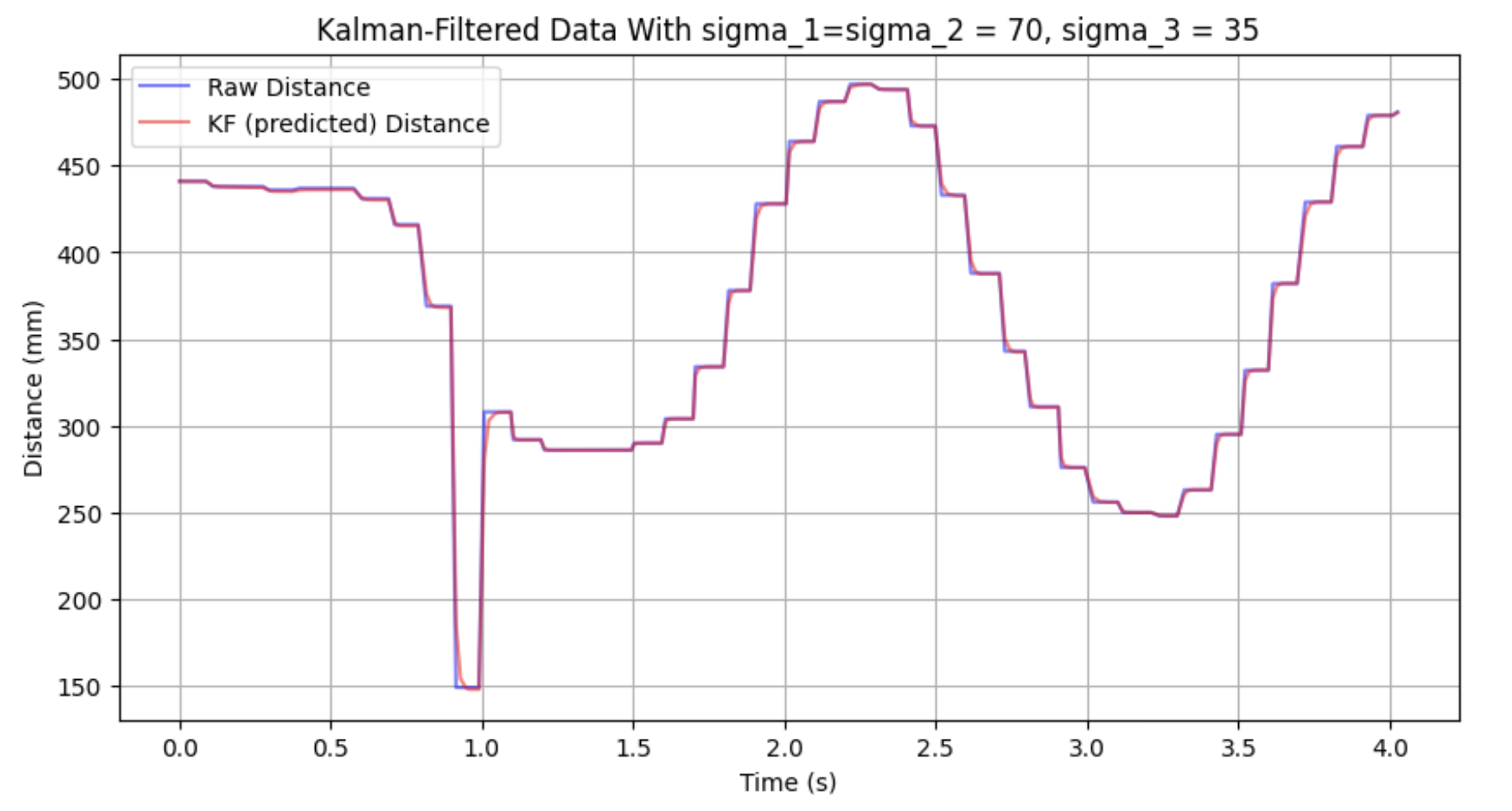
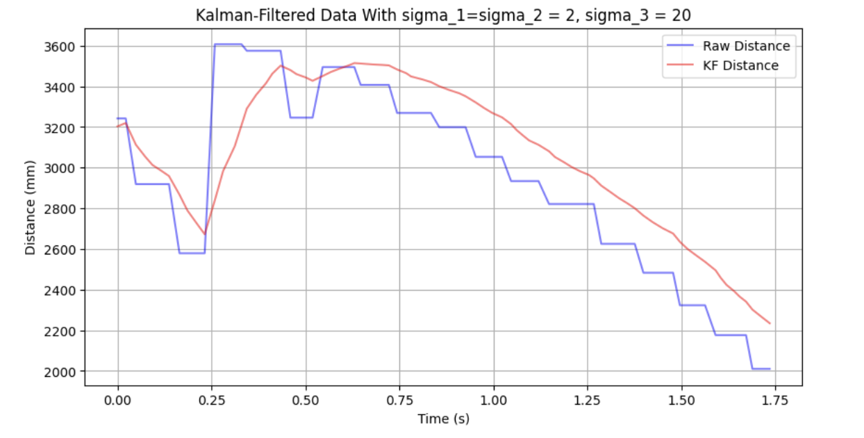
This is a bit tight to the raw data for my taste, Decreasing process noise (i.e. if I become more certain about the model I think my robot operates on, and less certain of my sensor data relative to the model), I get the following:

After tweaking the covariances some more, I was able to get the following filtered data, which appears to track the real distance pretty well:

Onboard Kalman Filter

To implement the Kalman filter on my robot, I wrote a function kalman_filter() which uses the BasicLinearAlgebra library for matrix math.

// state, uncertainties, measured val

struct KF_vars {
    Matrix<2,1> mu ;
    Matrix<2,2> sigma;
};

... 


KF_vars kalman_filter(Matrix<2,1> mu, Matrix<2, 2> sigma, Matrix<1,1>  u, Matrix<1,1>  y){

    // PREDICT

    Matrix<2,1> mu_p = Ad * (mu) + Bd * (u);
    
    Matrix<2,2> sigma_p = Ad * sigma * ~Ad + sigma_u;   

    // UPDATE

    Matrix<1,1> sigma_m =  (C * sigma_p * ~C) + sigma_z;

    Matrix<1,1> sigma_m_inv = sigma_m;

    Matrix<1,1> sigma_m_inv = {1/sigma_m(0)}; // use scalar inverse instead

    Matrix<2,1> kkf_gain =  sigma_p * ~C * sigma_m_inv ; 

    Matrix<1,1> y_m =   y -  ( C * mu_p);


    Matrix<2,1> mu_out = mu_p + kkf_gain * y_m ;
    
    Matrix<2,2> sigma_out = I  - kkf_gain * C * sigma_p ; 

    // FORMAT FOR OUTPUT

    KF_vars out;

    out.mu = mu_out;
    out.sigma = sigma_out;

    return out;
  
}

I didn't use the BasicLinearAlgebra Inverse() function as I found it didn't invert the 1x1 sigma_m correctly. It was pretty simple to just take the scalar inverse, though.

I did some testing on just the TOF (no motor input) and found really promising results with the above uncertanties: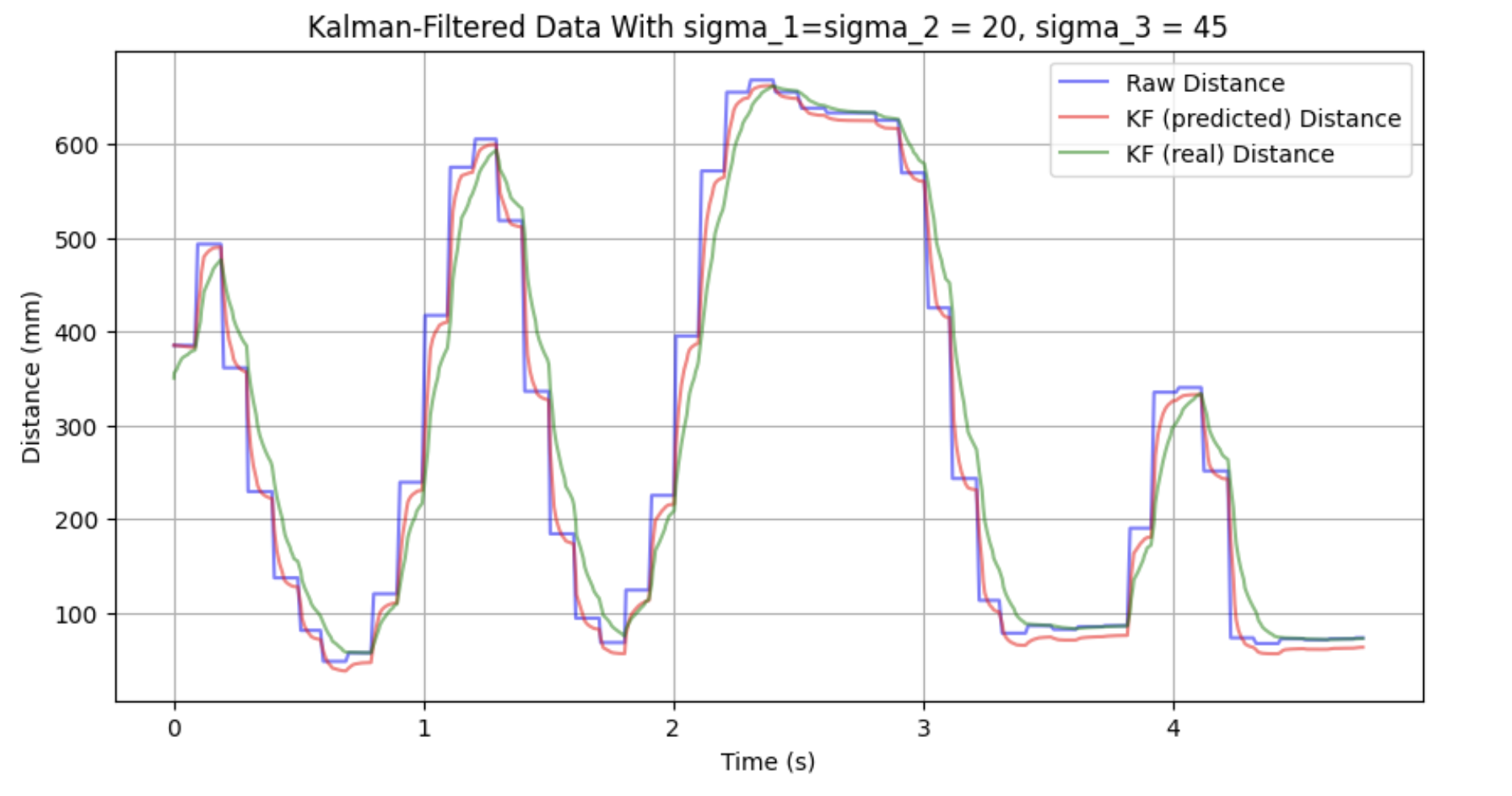

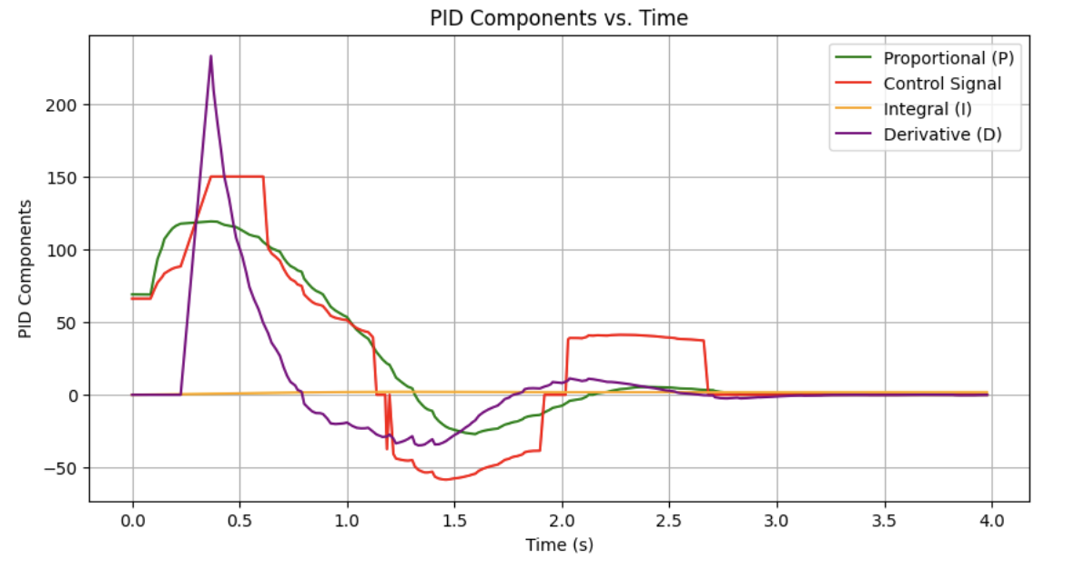
As a sanity check, I tried modifying my gains in a similar manner to the above, and got the following responses: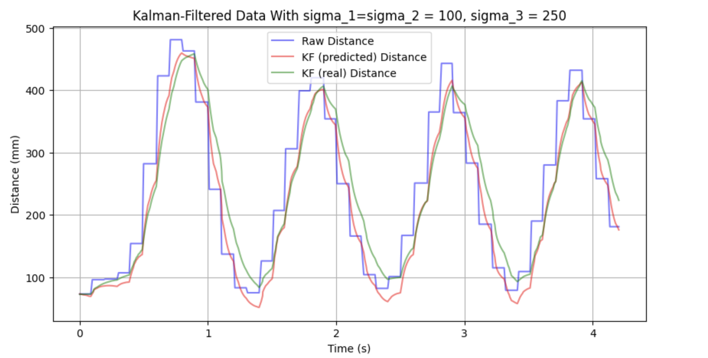

Although there are a few differences between the measured and predicted Kalman filter data, they have similar enough characteristics that I don't think the controller will have any trouble.

This one was a bit heavy on the P gain, but showcases the smoothness of the filter well:

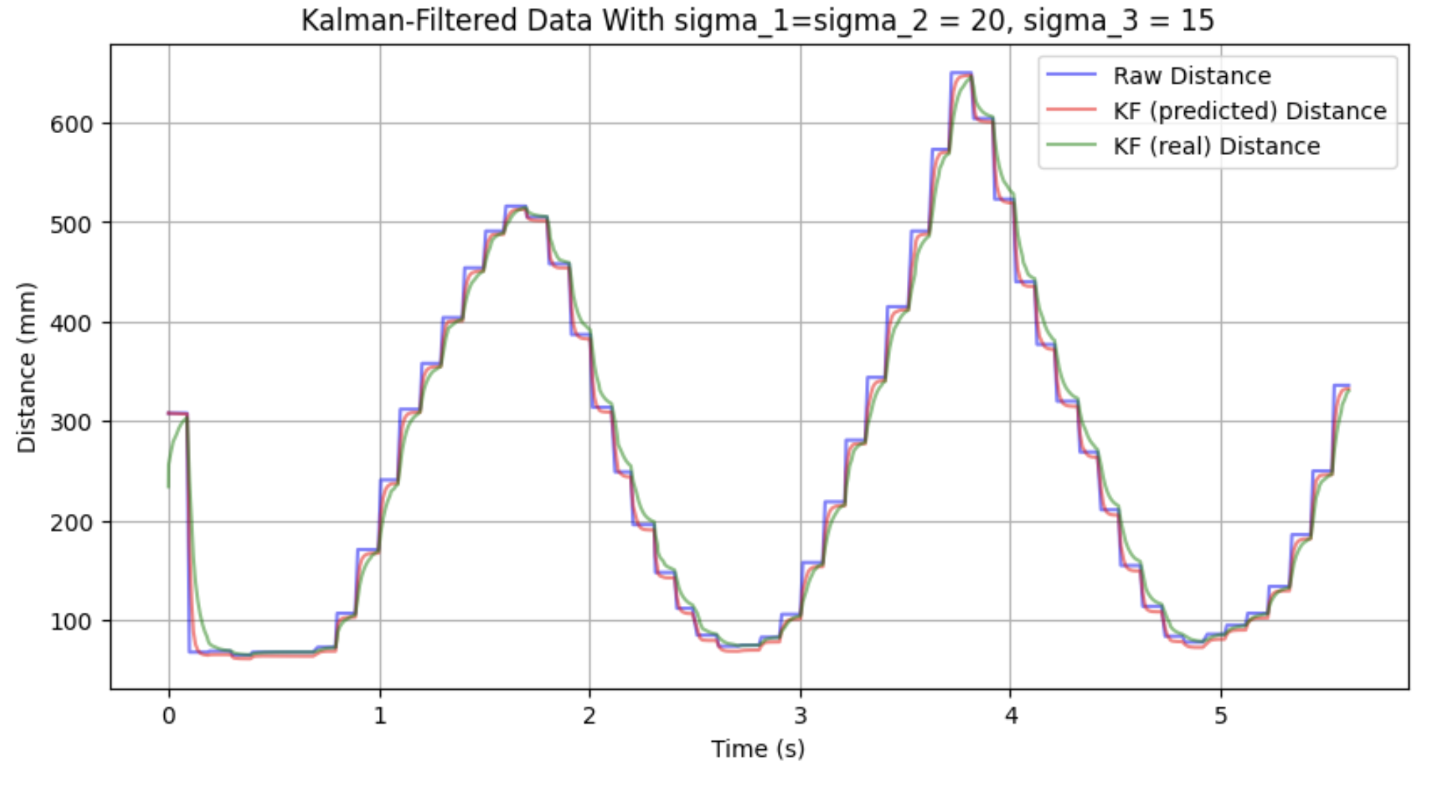
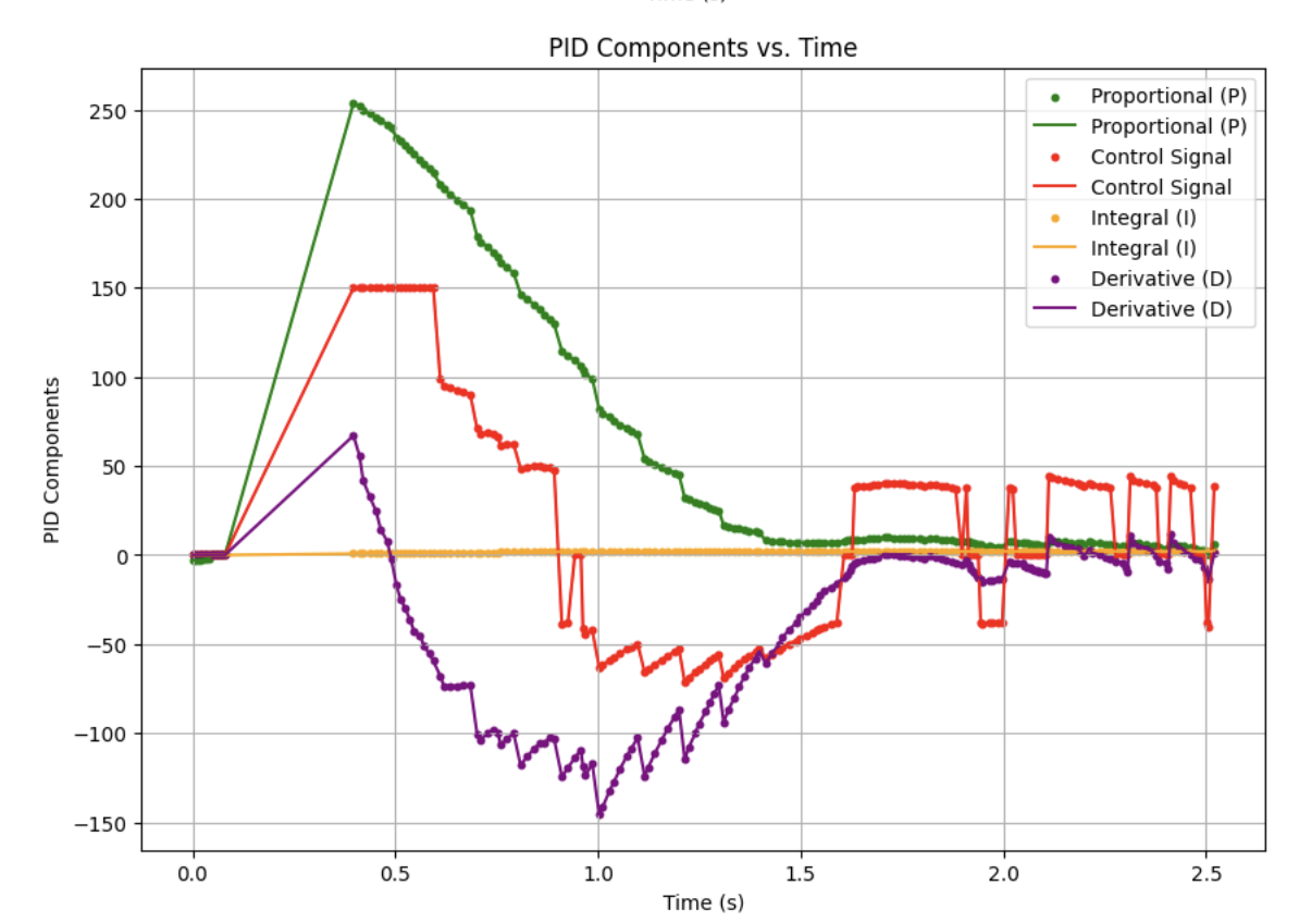
After some tuning, I got the following response:

Note: Fix of the initial TOF zero values coming soon!

Collaborations

I worked with Lucca Correia and Trevor Dales extensively. I used ChatGPT to help with curve fitting and generating nice plots and looked at Stephan's site for some rationale on initial estimates.

Next: Lab 8